Investigating Conditions Pre- and Post- Wildfire

Motivation

Wildfires have immense impacts on our ecosystems by destroying vegetation, disrupting wildlife and even altering the soil compositions. Understanding wildfires can help to predict and mitigate these environmental impacts, aiding in conservation efforts. Collecting data on the area before, during and after fires can display indicators of potential fire risks and the recovery of the land afterwards. Climate engine allows us to visualize this using remote sensing data and climate data.

For this tutorial, we focused on Camp Fleischmann, which was a summer camp operated by the Nevada Area Council of the Boy Scouts of America (today Scouting America) from 1953-2021 outside of Chester, California near Lassen Volcanic National Park. It was closed indefinitely following extensive damage in the Dixie Fire in July-August 2021. Other than minor clean-up work, very little recovery and reconstruction has been done, and no units have camped there. Unlike nearby areas, no heavy logging has been done in the camp. We will walk through understanding conditions prior to and following the fire. 

About the Datasets

We used two datasets to investigate the Dixie Fire, which started on July 13, 2021. 

GridMET is a climate reanalysis dataset that offers daily maps of meteorological variables, including precipitation, and temperature. In our analysis of the Dixie wildfire, we use GridMET Drought data to examine the role of drought prior to the fire. This helps identify potential fire risk indicators, such as short-term or long-term drought conditions. 

Landsat, a satellite mission jointly operated by the US Geological Survey and NASA, has been capturing imagery of Earth's surface since 1984. This makes it one of the longest-standing environmental datasets available. We used Landsat data to analyze the Normalized Burn Ratio Index (NBR) which references healthy vegetation or bare ground conditions. We also used the Normalized Difference Vegetation Index (NDVI), another indicator of vegetation health and productivity.

Mapping Drought Conditions using GridMET Drought

Wildfire activity is directly connected to weather and climate variations. Studies have linked drought indicators to wildfire occurrence in the Western US (McEvoy et al., 2019). Some drought index predictors include Palmer Drought Severity Index (PDSI) and Evaporative Demand Drought Index (EDDI).

(PDSI) is a standard index that examines dryness of soil. It ranges between values of -10 to 10. EDDI is described as a useful tool for monitoring “flash droughts” short-term, rapidly evolving droughts. EDDI examines how anomalous the atmospheric evaporative demand is for a location and time period (e.g. 14 days, 30 days, 60 days, etc.). EDDI is better for detecting short-term drought events compared to PDSI which can lag in response to quick changes in drought conditions.

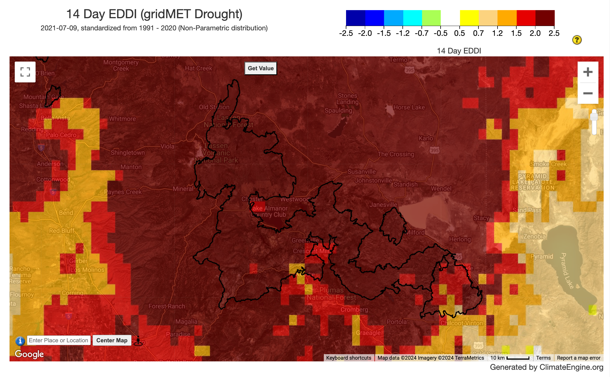
To produce the drought maps, open the Climate Engine App and navigate to the ‘Make Map’ tab. The first thing we are going to do is update the ‘Dataset’ drop-down to be GridMET Drought - 4km - Pentad and the ‘Variable’ drop-down to be 14 Day EDDI. Once we have our variable information updated, the Processing section will automatically update with the  ‘Statistic’ dropdown updating to ‘No Statistic’ and the ‘Calculation’ updating to ‘Standardized Index’. Lastly, we move to the Time Period section and select an ‘End Date’ of 2021-07-14, which was the closest date of data prior to the fire. Then, we click ‘Get Map Layer’. For visualization purposes, click the ‘Layers’ dropdown above the map and navigate to the US Fire Perimeters Layers. Turn on the 2021 perimeters, and head to the location of the Dixie fire.

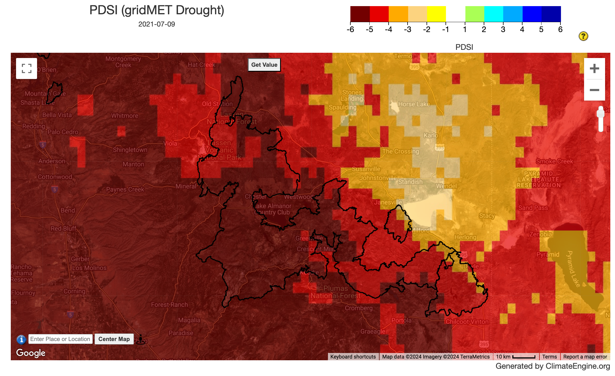
Next, for making the PDSI map we will repeat the same steps with a single change. In the Variable section, we will update the ‘Variable’ drop-down to PDSI and then click ‘Get Map Layer’.

Charting Drought Pre-Fire

After getting a spatial snapshot of drought prior to the fire, we will look at how drought changed over the five months leading up to the fire. To do this, we will switch tabs on the left side of the app from ‘Make Map’ to ‘Make Graph’. First, we will update the Time Series Calculation section by switching from ‘One Variable Analysis’ to ‘Two Variable Analysis’. Second, we will move to the Region section and change the drop-down from ‘Point’ to ‘US Fire Perimeter Layers’ . Two more drop-downs will populate. For the first, we will select the year of interest, i.e. 2021. For the second, we will select the name of the fire, i.e. DIXIE. Last, we will move to the Variable section. For Variable 1, we will make sure the ‘Type’ drop-down is Climate & Hydrology, the ‘Dataset’ drop-down is GridMET Drought - 4km - Pentad, and the ‘Variable’ drop-down is 14 Day EDDI. Then we will update the Time Period with a ‘Start Date’ of 2021-02-09 and ‘End_date’ of 2021-07-09. For Variable 2, we will repeat the same process except selecting PDSI in the ‘Variable’ drop-down.

After filling out the parameters, click ‘Get Time Series’ the resulting chart will output to the right. From the chart, we can see that the EDDI data displayed 5 spikes in the previous 5 months leading up to the fire. The largest short-term drought was just before the fire. The PDSI also indicated a worsening drought leading up to the fire.

Mapping Post-fire Impacts and Recovery

Landsat-derived indices such as the Normalized Burn Ratio (NBR), differenced NBR (dNBR), Normalized Difference Vegetation Index (NDVI), and Land Surface Temperature (LST) provide critical tools for evaluating post-fire landscapes. NBR is widely used to assess burn severity by highlighting changes in vegetation and soil reflectance, with high values indicating healthy vegetation and low values suggesting fire-affected areas. By calculating the dNBR, which measures the difference between pre-fire and post-fire NBR, researchers can quantify the severity and extent of burn impacts. NDVI complements this analysis by monitoring vegetation recovery over time, as it tracks changes in plant greenness and productivity. LST offers additional insight into thermal changes in the landscape, often showing elevated temperatures in fire-scarred regions due to reduced vegetation cover and altered surface properties. 

To produce the burn severity maps, we will first navigate to the ‘Make Map’ tab. We will start off by updating the ‘Type’ drop-down to Remote Sensing. By switching the ‘Type’, the ‘Dataset’ selection will update.  We will leave it on Landsat 5/7/8/9 SR - 30m. Next we will update the ‘Variable’ to NBR. We will keep the Processing sections as is, and move to the Time Period Section. We will update the Start Date to 2021-08-07 which is right after the fire was mostly contained, and update the End Date to 2021-08-31. Then we click ‘Get Map Layer’ and zoom into the area around Camp Fleischmann. We see a significant number of low NBR value pixels throughout the camp area.

Next, to get at burn severity we will map dNBR. To do this, we will update the ‘Calculation’ drop-down from Values to Difference from Average Conditions. This will cause  ‘Year Range for Historical Avg/Distribution’ dropdowns to be added to the Time Period section. Then we click ‘Get Map Layer’. This map shows patches (red) of high changes in NBR relative to the pre-fire conditions.

Charting Post-fire Impacts and Recovery

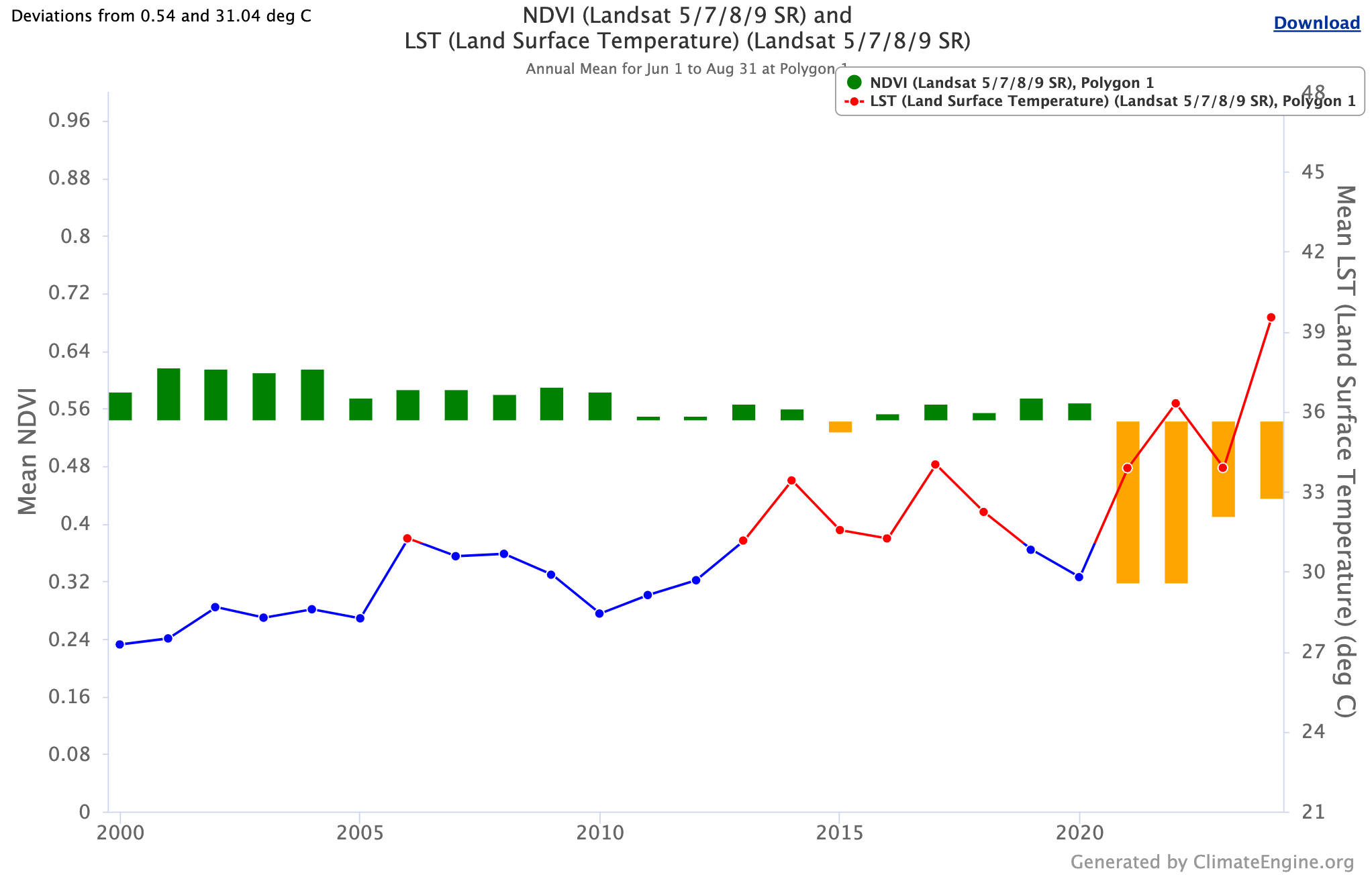
After visualizing the impacts of the fire, we will look at how different indicators of vegetation health have changed over time pre- and post- fire. This will help give insight into how the area is recovering, noting that there are only three years of data post-fire. To start, we will switch to the ‘Make Graph’ tab. In the Time Series Calculation section, we will update the Native Time Series to Summary Time Series and ‘One Variable Analysis’ to a ‘Two Variable Analysis’. Next, we move to the Region section and update the drop-down to Polygon. We are then able to draw a polygon surrounding the camp to summarize the data over.

Once we have our polygon, we can update the Variable 1 and Variable 2 of the Variable section. For Variable 1, we will update ‘Type’ to Remote Sensing, this will automatically update ‘Dataset’ to Landsat 5/7/8/9 SR - 30m, and ‘Variable’ to NDVI. This is what we want to keep for Variable 1. We will pick the JJA time period and update the year range to 2000 to 2024. For Variable 2, we will update the ‘Type’ to Remote Sensing which will automatically update ‘Dataset’ to Landsat 5/7/8/9 SR - 30m. We will then update the ‘Variable’ to LST. Lastly, we will update the Time Period to match the selection for Variable 1 and click ‘Get Time Series’.